e/D - field data versus Moody

Reviewing Moody's 1944 paper.  Moody, L. F. (1944). "Friction factors for pipe flow." Trans. ASME, 66:671-678.

His Fig. 2 is a look up for e/D values. I plotted the Winter/Summer friction factor numbers on the figure and the e/D values range as thus:

or

RC: 0.00015 to 0.0006
CC: 0.0005 to 0.00112

In comparison, previous Master's work found e/D values for

RC: 0.000075 to 0.00045
CC: 0.000075 to 0.00095

These are significantly smaller values for the friction factors we see on the pipelines.These values were based on Colebrook/White equation.

I'm seeing Reynolds numbers in the 10^4 (1L) to 10^5 region. I think C/W is only good in the transition region. I'll need to verify.

One of the things I do like that Moody did was to plot all the different equations (Von Karman/ Pandlt/Nikraduse, Colebrook, Rouse) against each other.

Had an "aha" moment.

We pump in the transition zone (purple box below). I've known this for a while.

Moody also discussed how difficult it is to come up with a real absolute roughness value. The values the industry uses are the ones based on the sand grain sizes from Nikraduse. Moody indicates the engineer should rely instead on the hydraulic roughness, or e/D.

From Moody:

When the thickness of the laminar layer, which decreases with increasing Reynolds number, becomes so small compared to the surface irregularities that the laminar flow is broken up into turbulence, the flow conditions pass over into the zone of "rough pipes" with complete turbulence established practically throughout the flow. Viscous forces then become negligible compared to inertia forces, and f ceceses to be a function of the Reynolds number and depends only upon the relative roughness, giving horizontal lines of constant f in the chart.

Which means the evidence I see with the cyclical f versus Reynolds numbers values DO have significant viscous forces at work. So can this mean that we could have differing flow regimes based on water properties of the water (density/temperature/etc)?

Moody also mentioned the results of Colebrook plots that produced results from an Ontario large diameter penstock. The f v. Re values put the results close to very smooth pipe.

Another item to vet out is the absolute roughness/boundary layer values. Appearently, Moody based his work on a constant value 6.08, which is considered somewhat high.

Also, Rouse showed the e/D values Colebrook found, fall within experimental scatter.

So now I'm starting to think about how this relates to biofilm. These values are all based on static roughness measurements. I think I may want to consider abandoning the pipe roughness v. biofilm roughness in favor for a dynamic hydraulic roughness of the pipe.

I do see cycical variation. Do I tie it to temperature? Viscocities? I lean toward viscosity since previous work showed temperature was somewhat independent of other water properties (the linear regression class work).

Could this be significant work?

Literature Review.

Friction factor is independent of the Reynolds number (Darcy, H. : Recherches experimentales relatives au mouvement de 1'eau dans les tuyaux. Memoires a l'Academie d. Sciences de 1'Institute 
imperial de France, Bd. 15, 1858, p. 141.)

Relative roughness (k/r) where k is absolute roughness. (v. Mises, R.: Elemente der technischen Hydrodynamik. Leipzig, B. G. Teubner 1914.)

Since kinematic viscosity impacts the Reynolds number, I would like to understand what kinematic viscosity really means.

Kinematics: Geometric in nature, defines motion without regard to forces that cause motion or result from motion.

Kinematic viscosity is traditionally measured by noting the time taken for a fluid sample to travel through an orifice in a capillary under the force of gravity.

Every type of fluid possesses differing amounts of resistances against deformation. The measure of that resistance is called viscosity. Viscosity expresses the fluid’s resistance against either tensional stress, or shear stress.

Fluid Dynamics

So I got my Experimental Fluid Mechanics book and started on page 1.

Ugh.

Thought I didn't have to deal with thermodynamics ever again, but it totally makes sense that it is a big part of it.

First thing off the bat: total internal energy is a function of entropy and density.

e = e(s, rho)

Also I watched this course

Problem Statement - first draft

This is a first attempt at a problem statement.

Standard design parameters used by engineers for pipeline design uses static hydraulic conditions between new pipe and old pipe by varying friction factors. Previous work has found hydraulic conditions cyclically vary during one calendar year to where energy loss ranges change from values equal to either new pipe (winter conditions) or aged pipe (summer conditions) friction factor values. Thus, there are two different types of roughness: pipe roughness and biofilm roughness. Pipe roughness is based on actual rugosity of the pipe wall. Biofilm roughness is based on the seasonal variations of friction factor, which directly quantifies energy loss, that can be attributed to biofilm growth. 

Previous work on pipe roughness for large diameter pipe, or pipe that is 60-inches in diameter or larger, found that when experimental results were plotted on the traditional Moody diagram, the ratio of the roughness of the pipe to the inertial forces captured with Reynolds number does not follow the classic model used with the Moody diagram for large diameter pipe. 

Biofilm is considered a viscoelastic medium in that the thickness can vary. Previous work has found velocity of the water in the conduit has an inverse relationship with the thickness of biofilm. The higher the velocity, the thinner the biofilm and visa versa. Biofilm thickness is also impacted by environmental conditions of the water within the pipe. An environmental process which can directly impact pipe roughness over time may be due to the presence of biofilm in the pipeline as evidence shows that nitrification occurs within the pipeline. This process lowers the pH of the water in the line which then can put any cementitious lining in jeopardy of increasing pipe roughness since the Langlier Saturation Index (LSI) will be negative, which indicates calcium carbonate (CaCO₃) dissolves in water. In the system studied, the limestone aggregate as well as the sand contain high amounts of CaCO₃ which have been eroded over time increasing the rugosity of the inner pipe wall.

This paper will try to 

Establish the difference between pipe hydraulic roughness and biofilm roughness in long large diameter raw water transmission pipeline.

Establish there is a relationship between algal growth and increased friction factor values and in turn, determine the change in the hydraulic roughness of the pipe. 

Establish if there is a spacial and time relationship between LSI, pipe rugosity, and biofilm growth.

More basics

Reynolds number is the ratio between inertial and viscous forces of a fluid.

Here's a link to a lecture that goes over more mechanic basics. I've been reviewing this one.

I like how it goes over Reynolds numbers pictorially.

Came across this in reading the BR Tech memo

What experimentation indicates that frictional resistance varies at the first power of the velocity and the second power of the pipe diameter?

Back to shear wall stress basics

I'm pretty exhausted tonight, but I did dust off some basic review.

Headloss can be found using the following equation.

 where:

Combining that equation with the Darcy-Weisbach yields the following for the wall shear stress:

Thus the wall shear stress is located at the wall of the pipe, where the velocities will be smaller than what is found towards the center.

So biofouling makes the wall shear stress increase when the film gets thicker. This would effect flow rates as it will impact the velocity distribution profile. So I can now use the wall shear equation to relate it to velocity.  Right now, I get flow rates based on differential pressures in a venturi tube.

 These are based on set diameters and distances within the venturi tube. I need to review how these go back into SCADA with the Pressure Indicating Transducers (PIT). The idea is the flow rate is a true flow rate measurement and I can use the venturi meter to come up with a true velocity based on a fixed diameter. The thought is that biofilm decreases the area of the pipe. Could I get a correlation of biofilm thickness to the pipe wall with this analysis? If I used the pressure transducers I have out on the pipeline, could I come up with an aggregated thickness (like a mean thickness value)?

Non-neutonian fluids are fluids like toothpaste and cornstarch mixtures - i.e. sludges. Sludges will tend to move in the laminar flow range. (Refer to email from colleague from the Day 1 post). While algal fouled water may have a higher viscosity value, it's not moving the regime into laminar territory. I do believe viscosity is at play, so this does have merit.

Nitrification and Carbonation of Pipe

3. Biogenic nitric acid The biogenic ammonia present in water environments stimulate the concrete corrosion caused by the biogenic nitric acid. The ammonization bacteria (urobacteria) decompose urea and cause the ammonia formation. Bacteria belonging to Nitrosomonas, Nitrosococcus, Nitrosospira and Nitrosolobus genera oxidize the ammonia to nitrous acid subsequently oxidized to nitric acid by Nitrobacter and Nitrococcusbacteria. This acid reacts with calcium compounds in the hardened cement paste to form the water-soluble calcium nitrate, easily rinsed from the concrete structure[17]. It has been shown that the biogenic nitric acid produced by the nitrifying bacteria causes severe corrosion of the mineral building materials. High cells numbers of the nitrifying bacteria were present on both historical sandstone buildings as well as on modern concrete buildings [8, 9].

We know we have Nitrification going on in the pipeline. Looks like we're generating nitric acid which is why we're getting high levels of concrete degradation.

Is there a way to determine this in the concrete samples of the pipe with the petrographic analysis? Can he test for calcium nitrate?

Fiber Optic and Biofilm Thickness

So I started looking over the DOE Biofilm website I posted yesterday.

I found a very cool side link for research ongoing for acoustic microscopy for biofilm. In a previous post I mused about how to quantify/link biofilm thickness with velocity/viscosity of the water. This is definitely something I need to look at. From what I can see, it uses Ultrasonic Technology (UT).

But wait! When I went to ASCE Pipelines this year in Baltimore, I tagged along with a colleague to go to a forum on fiber optic monitoring for pipelines. I have to admit, I was really excited by what I came across. Dr. Jey Jeyapalan was the organizer and is championing using fiber optic within the ASTM F36 committees.

Another item brought up in the conference was using acoustical fiber optics to be able to hear when a wire breaks on a prestressed concrete cylinder pipe.

So, is there a way to combine fiber optic with the UT technology PNNL is developing to help determine biofilm thickness? Can you use FO to measure viscosity, too?

Found a reference to a thesis that was written in 1990: "Thickness and density measurements in biofilm with a fiber optic sensor", Thesis Defense by Gabriele Walser, MS.

Major finding: The results for biofilm grown in the rotating disk reactor indicate that biofilm thickness depends on shear stress.

Which supports what I was talking about earlier. Looks like there's been some serious research on this. Get to go chase down research. I have trouble with it because I end up chasing lots of rabbit trails.

Here's another idea:

Characterization of the effects of low power pulsed vibration energy on biofouling inhibition in water piping systems

Can you use FO to induce a pulsed vibration to keep biofilm from establishing?

Dusting off V. 4 of Master's Thesis

Okay, so I cracked my version 4 (out of 9!) masters thesis and saw that it was 17 M large (the final was 6 M)

I had hypothesized using different methods of indicating there is bio-activity in the pipeline.

Monitor Chlorine Residual - hypothesized faster chlorine decay means there is higher biological activity.

I could go more into chlorine decay with regard to biological activity but I think its already been established academically. The question, though, is how much is due to the biofilm and how much is due to algal activity. I can chase that rabbit trail, but my interests lie with the hydraulics. So why worry about biofilm growth? Because it directly impacts pumping systems. When we are designing pump stations

So a biofilm is a mass of cells located at solid/liquid boundaries that are held together with "a matrix of extracellular polymeric substance (EPS)". It's the EPS that really protects the bacterial cells and allows the cells to grow into colonies.

I do know that the two types of algae that are most prevalent when friction factors are high are blue-greens and diatoms. Here are some charts showing what types of algae has been found in both Cedar Creek and Richland Chambers.

But when I compared the information to friction factor, there is a definite correlation

I wish I had more frequent algal data. But this is still pretty good to see.

So I feel like I may be going in a direction. Quantify viscoelasticity of biofim based on velocity - could it relate to a hydraulic roughness?

From earlier unpublished thesis work:

The only immediate changes to the friction factor occur with a pump combination change. The change could be due to a change in velocity, which can affect the biofilm thickness. Faster flows yield lower friction factors and visa-versa. The change in friction factors due to pump combinations could be supporting evidence that the biofilm performs as a viscoelastic medium. Biofilm formation could also be disrupted during pump changes and the biofilm configurations may be rearranged due to higher shear stresses occurring at the pipe wall during pump combination changes.The only immediate changes to the friction factor occur with a pump combination change. The change could be due to a change in velocity, which can affect the biofilm thickness. Faster flows yield lower friction factors and visa-versa. The change in friction factors due to pump combinations could be supporting evidence that the biofilm performs as a viscoelastic medium. Biofilm formation could also be disrupted during pump changes and the biofilm configurations may be rearranged due to higher shear stresses occurring at the pipe wall during pump combination changes.

Which gets me back to basics. 

So, do I try to quantify viscosity of water to algal count and tie it to friction factor? Or better yet, try to come up with a way to relate velocity/viscosity to hydraulic roughness. Since the biofilm is viscoelastic, can there be some type of factor that can relate hydraulic roughness to velocity?

Again, this would only be for large diameter pipe.

Viscosity and Algae

Terrible.

Okay, so I did brush up on very BASIC fluid mechanics.

One thing that was prevalent in my previous research is how much viscosity impacted friction flow. From what I have found, viscosity has an inverse relationship with temperature - which is counter to what I had in my mind since friction factors change from summer to winter. I thought viscosity would have a direct relationship with visocity - ie, viscosity goes up, friction factor goes up.

So something else is at play here. I have some evidence that the spike in algal growth in the lakes coincide with the increase of friction factor - it's not really pronounced, but I do find we see an increase in the times where the lakes are turning over. When lakes turn over, more nutrients are stirred up in the lake. Could this be feeding the biofilm down the line? Can I quantify the types of biofilm to see what nutrients they need? Does the type of biofilm change from lake to lake, i.e., is the biofilm in RC similar to the biofilm in CC? Does nitrification occur in RC in the same area that it does in CC? Is this time/velocity related, which could impact colony locations.

So I need to get a program going to measure viscosity of lake water. I would like to do it on the same day the algal counts are made.

Resource: http://www.hydramotion.com/portable.html

I found a book that has a lot of good information regarding how some experimental fluid mechanics get done. I found it when running a google search on "how to measure viscosity of water"

Springer Handbook of Experimental Fluid Mechanics / Edition 1

• by Cameron Tropea
• Other Format
• (2007)

It's at Barnes and Noble.

Documenting Environmental Info

I definitely agree this system is complicated, with lots of factors at play.

In looking at the data we have been collecting this year a few additional thoughts:

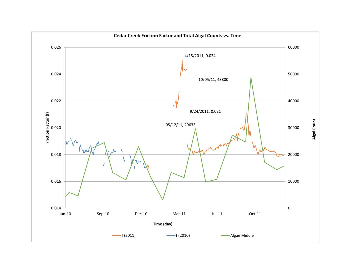
1)      It appears flow rate (detention time) in the pipeline is a very large factor. I have attached some graphs comparing this summer to last year.  These data show that we are losing chloramine at almost the same rate, not only between this year and last year, but also between RC and CC lines. I am working on compiling more of this data that we have collected and plan to plot on the same graph so we can see the trends better. Now that we are (or planning to be) pumping at higher flow rates, we will see if this trend holds true.

2)      From some other work we did, we can show that nitrifiers are present - We see much less chloramine loss in pipeline samples that are filter sterilized.

3)      We got TOC samples back from our last sample event (8/19/2015) and TOC is much greater this year in Cedar Creek. This will lead likely to higher chloramine demands. I think this may also result in lower conversion efficiency. It has been difficult to gauge this year because of the low flows, but now that we are pumping at higher rates we will be able to compare this. TOC results are below:

a.       Cedar Creek – 5.8 (in 2014) vs. 7.5 (2015)

b.      Richland Chambers – 4.5 – 5.0 (in 2014) vs. 4.8

c.       Benbrook – 4.7 (in 2014) vs. 4.9

4)      From what I have seen, DO varies diurnally at the intakes due to algae, even though we aren’t pulling right off of the surface of the lakes – this will impact DO levels in the pipelines. As mentioned, biological activity consumes DO. For example during nitrification:

a.       AOB convert ammonia to nitrite – this process consumes 3.16 mg/L DO per mg of ammonia as N

b.      NOB convert nitrite to nitrate – this process consumes 1.1 mg/L DO per mg of nitrite as N

c.       So when we have complete nitrification in the pipeline (all ammonia taken to nitrate) for each mg/L of N, we will lose 4.24 mg/L of DO.

d.      We are currently dosing about 1 mg/L of ammonia to form chloramines; not all of this will be converted to ammonia when the chloramines decompose, but a significant fraction may. I am working on estimating how much ammonia we can expect to be available for nitrification.

e.      It would be interesting to track DO based on travel time (like we did for chloramine loss) to see if we see the DO loss at the same approximate travel time in the pipe and if we see a difference in DO loss in years when chloramines weren’t fed to when they were. I imagine as we travel down the pipeline, the biological community changes based on what “food” is present. However,  it would be interesting to see if the shift in community will result in more or less DO being consumed when we compare feeding chloramines to not feeding chloramines or comparing low flow rates (this year) to high flow rates (last year) when we were feeding chloramines.

I plan to continue hashing this stuff out…….

Thanks,

Greg

From: David Marshall [mailto:David.Marshall@trwd.com]
Sent: Monday, August 31, 2015 10:03 AM
To: Shelly Hattan; Mark Ernst; Donna Stephens; Jason Gehrig; Rachel Ickert; Greg Pope; Robert Cullwell; Darryl Corbin; Troy Laman; Darrel Andrews; Chris Zachry; Alice Tu; Jim Gallovich
Subject: RE: Low Oxygen in the pipeline

A couple of other things to consider:

1.        BOD and COD are highest in the water column during the summer.  This year I would expect it to be greater than normal thanks to the nutrient slug from the floods.

2.       The diurnal swings of DO in the reservoir may influence what we are pumping.  Pumped water is slug flow, so if the time of sampling could be compared to the time it began to be pumped, the change may provide some insight.  For example, we start the sampling at the lake stations early in the day.  The wetwell is full of oxygen rich water since the lake has started photosynthesis, adding oxygen.   As the samplers move down the line, they encounter water that was pumped at night when the lake was fully in respiration.  

3.       Nitrification  may also be on the reservoir, as well as the pipeline.  http://www.google.com/url?sa=t&rct=j&q=&esrc=s&source=web&cd=1&cad=rja&uact=8&ved=0CCMQFjAAahUKEwiLkuP8ytPHAhWDWZIKHQtvDNE&url=http%3A%2F%2Fwww.pjoes.com%2Fpdf%2F13.4%2F415-424.pdf&ei=6WvkVcv5EoOzyQSL3rGIDQ&usg=AFQjCNE-5Ffq1ZbxN4O_29jwHZOKQHMLyg

The community in the pipeline and the chemistry is complex.

David H. Marshall, P.E.

Director of Engineering and Operations Support

Tarrant Regional Water District

800 East Northside Drive

Fort Worth, Texas 76102

Office: 817.720.4250

Cell: 817.475.0061

https://www.facebook.com/TarrantRegionalWaterDistrict

twitter @trwd_news

From: Shelly Hattan
Sent: Monday, August 31, 2015 8:27 AM
To: Mark Ernst; Donna Stephens; Jason Gehrig; David Marshall; Rachel Ickert; z Greg Pope; z Robert Cullwell; Darryl Corbin <DCorbin@carollo.com> (DCorbin@carollo.com); Troy Laman (TLaman@carollo.com); Darrel Andrews; Chris Zachry; Alice Tu; z Jim Gallovich
Subject: RE: Low Oxygen in the pipeline

My hypothesis is this:

·         Cooler temperatures = low biofilm activity.

·         Flow rate = differing biofilm thicknesses – the faster the velocity, the flatter the biofilm gets (viscoelasticity of biofilm)

·         DO = lowers with higher biofilm activity. We see a spike up in DO when we boost pumping (read: Ennis (25.5) and Waxahachie (43)) since the water has to recycle through the tanks. It’d be interesting to see what the DO is before entering the tanks and then after. Not sure if sampling was done on suction side or discharge.

I believe the algae in the water enters the pipe, respires and introduces CO2 in the water. With the algae data we have, it looks like we see a change when the blue-greens and the flagella (?) are highly active. I never did go back and try to correlate the algae data with your LSI results. Could prove to be interesting. The CO2 then gets used by bacteria to start growing – and I believe since we are nitrifying in between Ennis and Waxahachie, we have an Ammonia Oxidizing Bacteria strain in the pipe.  The AOB then starts using the oxygen, which brings down DO. The increase in CO2 also increase bicarbonate when combined with water (HCO3-). Bicarb then helps contribute to the carbonation occurring in the concrete core of the pipe – hence the loss of CaOH from our concrete (i.e. a direct result of low LSI’s). I plan on using the petrographic sampling program results to compare the material loss with the DO data to see if there’s any relationship I can tease out of it.

I believe the use of Chloramines helps in a number of ways:

Stabilizes biofilm growth. Compare the 2010 data with the 2012 data. DO loss should not be as dramatic. I think if we could maintain a residual higher than 1 (possibly around 2 to keep nitrification at bay), we’d see DO stay far more consistent. I found in my thesis work that the friction factor has an inverse relationship with DO, which I interpret as what I’m hypothesizing.

That’s my 2 cents worth. Also note, that RC looks like it behaves differently. I believe we have a different type of bacterial colony established there. I’d like to prove that out by sampling some blow offs – I believe we could close the butterfly valves and be able to scrape samples from inside the manway.

I’d love to hear something from our consultants to verify some of my thoughts.

From: Mark Ernst
Sent: Monday, August 31, 2015 7:57 AM
To: Shelly Hattan; Donna Stephens; Jason Gehrig; David Marshall; Rachel Ickert; z Greg Pope; z Robert Cullwell; Darryl Corbin <DCorbin@carollo.com> (DCorbin@carollo.com); Troy Laman (TLaman@carollo.com); Darrel Andrews; Chris Zachry; Alice Tu; z Jim Gallovich
Subject: RE: Low Oxygen in the pipeline

The graph below includes the last of July and the month of Aug in 2010 where the dissolved oxygen really tanked. If you look through all of these graphs and then cross your eyes and look through them again it seems like the dissolved oxygen in the line is a result of the temperature of water, flow rate in the pipeline and standing crop of biofilm in the pipeline.  I know the oxygen is negatively related to temperature, think it is positively related to flow and an guessing it is negatively related to biofilm.  Be real cool to quantify this!

From: Shelly Hattan
Sent: Friday, August 28, 2015 3:37 PM
To: Donna Stephens; Jason Gehrig; Mark Ernst; David Marshall; Rachel Ickert; z Greg Pope; z Robert Cullwell; Darryl Corbin <DCorbin@carollo.com> (DCorbin@carollo.com); Troy Laman (TLaman@carollo.com); Darrel Andrews; Chris Zachry; Alice Tu; z Jim Gallovich
Subject: RE: Low Oxygen in the pipeline

The LSI study had some really good data on this:

2010

2011

2012

2013

From: Donna Stephens
Sent: Friday, August 28, 2015 3:06 PM
To: Jason Gehrig; Mark Ernst; David Marshall; Rachel Ickert; z Greg Pope; z Robert Cullwell; Darryl Corbin <DCorbin@carollo.com> (DCorbin@carollo.com); Troy Laman (TLaman@carollo.com); Darrel Andrews; Chris Zachry; Alice Tu; z Jim Gallovich; Shelly Hattan
Subject: RE: Low Oxygen in the pipeline

Thanks Mark,

Do we know the depth (in the reservoirs) that the water becomes hypoxic, anoxic, anaerobic?

The latest Zebra Mussel video post from TPWD…

http://youtu.be/zGJIbQ9WOt4.

Donna Stephens | Infrastructure Engineering Services

Tarrant Regional Water District  | Direct: 817-720-4251

From: Jason Gehrig
Sent: Friday, August 28, 2015 1:32 PM
To: Mark Ernst; David Marshall; Rachel Ickert; z Greg Pope; z Robert Cullwell; Darryl Corbin <DCorbin@carollo.com> (DCorbin@carollo.com); Troy Laman (TLaman@carollo.com); Darrel Andrews; Chris Zachry; Donna Stephens; Alice Tu; z Jim Gallovich; Shelly Hattan
Subject: RE: Low Oxygen in the pipeline

This looks interesting Mark.  If ZM’s won’t attach in <2 DO environments, perhaps we could develop a zebra mussel/biofilm control approach where min 0.3 to 0.5 chloramine residuals throughout the entire system-wide wouldn’t be required; but rather only in areas of the pipeline where DO’s are expected to exceed 2 mg/L. This would probably meet our biofilm control needs at the same time since we already chloramine feed there, at least in the longer stretches of higher head pumping (i.e. lake ps’s to Wax or so).  Adding chloramine feed at BB would still be needed but boosting requirements could be re-analyzed.

A good review of our seasonal DO data in our pipeline might shed additional light.

Thanks,

Jason

Also good info on hypoxic vs anoxic vs anaerobic as well

From: Mark Ernst
Sent: Friday, August 28, 2015 11:45 AM
To: Jason Gehrig; David Marshall; Rachel Ickert; z Greg Pope; z Robert Cullwell; Darryl Corbin <DCorbin@carollo.com> (DCorbin@carollo.com); Troy Laman (TLaman@carollo.com); Darrel Andrews; Chris Zachry; Donna Stephens
Subject: Low Oxygen in the pipeline

Interesting paper on the tolerance of zebra mussels to low dissolved oxygen levels.  The paper talks about “hypoxic levels” of dissolved oxygen which are defined as less than 2 mg/L  (Anoxic levels are less than 0.5 mg/L).  The results show that at  25 C (77 F) mean survival of zebra mussel adults was 2 to 3 days under hypoxic conditions.  Downstream from Wax Pump Station we get these conditions for about 2 months.

Yesterday at Midlothian Hill the dissolved oxygen in the CC line was .26 mg/L and in the RC line was .22 mg/L  at 29 C (84 F).  This was maintained to the KBR structures. I think we have an environment that is not suitable for zebra mussel infestation.

Catch-22

The loss of oxygen in the pipeline downstream of Wax may be accelerated by biofilm growth and bulk bacterial growth.   If we boost chlorine in the Wax area to reduce biofilm in the line downstream to KBR as a measure to reduce pipeline friction, then dissolved oxygen may remain high enough for zebra mussels. 

Some suggest we have a similar dilemma with our bottom aeration of the intake areas at Lake Benbrook and Lake Bridgeport, where we might be creating a habitat for zebras where there was once not one.  I don’t think so, our data from this summer at Bridgeport shows that even with our new diffuser configuration we are still going anoxic near the bottom, however we are not going anerobic.  Anerobic is where all the dissolved oxygen is gone and bacteria start to scavenge oxygen from molecules like SO₄ and make H₂S.  So, no new zebra mussel habitat and a reduced amount of anerobic bad boys.

Welcome your thoughts on this.

Mark R. Ernst

TRWD

817-999-9832 cell

817-237-8585 office

Day Three

Okay, so I didn't write yesterday, but I feel like I had a good excuse. I had a concrete pour that when way south early, early today - i.e. I've had 3 hours of sleep in 48 hours. Bleh.

Anyway, I did think about some of the fundamentals, but I didn't research it.

There's a relationship between hydraulic roughness and shear stress. I need to learn more about this. That's why next semester I want to take Fluid Dynamics from the ME department. I also want to take a boundary layer class from the ME's as well, but they don't have internet classes right now.

So, my thought is to really try to find a relationship between the two for large diameter pipe (and yes, I recognize this is very Polyanna-ish at this time, but that's what free writing is all about).

I met up with a consultant who has good connections with the North Texas Municipal Water District (NTMWD). They have large diameter pipe, do not chloraminate, and have zebra mussels. I'd like to reach out to them to see if I can get seasonal information. He mentioned that they are taking data every 15 minutes (which, based on the work for the Thesis, I found to be not very useful information - the data is really much more stable than what I originally thought.

So, I have to really look at that relationship.

Also, there are some items I would like to consider as well. It's a long shot (and I'll need to *really* go back to some of my old Biological Processes classes). When CH2M did some invasive species work to determine how to best determine chloramine dose, they took multiple data points based on TOC, Temperature of water, pH, etc. . .

They used Eureka to fit an equation to the data.

The result was somewhat controversial and not well received by my management. The equation showed that TOC had a much more prevalent role in chloramine residual performance.

This has never left me. These results also were discredited by an academic, and management. But I think there should be some more information collection to double check the results.

I also have wanted a conductivity meter at the lakes - I believe this can relate to TOC values. I need to research.

Action Item: TOC to Connectivity - will a connectivity meter be able to determine this on a regular basis.

Day 1 - 9/7/2015

I am currently reading "Writing Your Dissertation in Fifteen Minutes a Day" by Joan Boker, Ed.D. In it she outlines that I need to start writing everyday - just freewriting, in order to help me think.

So, this blog is my attempt to do that.

I wrote an email to a colleague I hold in high regard to somewhat give a direction for my research:

Friction factors for large diameter pipe change with velocity. Research for large pipe has been limited to 48” in the lab setting.

I would like to understand how the friction factor changes with change in velocity, hydraulic roughness, density of water, and kinematic viscosity in large diameter pipe. The data I collected in my Master’s work shows that  large pipe does not follow the traditional Moody diagram relationship. I found when plotting the calculated friction factor (from observed data) against the calculated Reynolds number, the ratio of the hydraulic roughness and the diameter of the pipe is smaller than what is shown on a traditional Moody diagram.

I suspect the hydraulic roughness calculation isn’t a good approximation for large diameter pipe because the boundary layer of the water/pipe interface may be smaller due to quick dissipation of shear stresses. In other words, the boundary layer in smaller pipe may be much larger due to the shear velocity being higher. I believe the larger diameter pipe has smaller boundary layers due the fact that the water has the ability to “normalize” in the large column of water.

To test this, I’d like to do computational fluid dynamic model of large diameter pipe and then calibrate it in the field with observed data points.

Since I have a number of different surface conditions, from new smooth pipe to highly pitted. I propose to identify locations where existing petrographic analysis reports give physical measurements of the depth of roughness. I can use these numbers to help identify a physical roughness value and use field measurements to be able to determine an average roughness. I can use kriging to help develop a hypsographic chart similar to what has been done by the Bureau of Reclamation by using a robotic 3D imaging system (http://gigamacro.com).

I got the following revisions from him:

Energy loss (i.e. Resulting from Friction at the wall) factors for large diameter pipe is dynamic and the magnitude of resulting resistance to fluid flow changes with not only the characteristics of the pipe wall, but the characteristics of the fluid and velocity. Empirical Research on the development of friction coefficient to estimate energy loss for large pipe has been limited to 48” in the lab setting. I would do a little work here to explain Darcy and Weisbach’s empirical work and the fundamental assumptions they made at the boundary and how it was decided to use the average velocity for turbulent flow estimates of head loss. I would be a little careful here because this is fundamental stuff and you would need to do tremendous data collection to truly evolve the established friction coefficients.

Suggest you read some of the early work (c. Late 1930s) and understand their basic assumptions. It is know that the cross sectional velocity profile in a full flowing pipe is not properly considered in the DW equation. Look at “internal flow systems” by D.S. Miller it’s a great reference with a significant amount of research performed by BHRA.

I would like to understand how the friction factor changes with change in velocity, hydraulic roughness, density of water, and kinematic viscosity in large diameter pipe. The data I collected in my Master’s work, show that the large pipe does not follow the traditional Moody diagram relationship. I found when plotting the calculated friction Factor (from observed data) against the calculated Reynolds number, the ratio of the hydraulic roughness (this is a measured value and as a result the ratio is a known, a given) and the diameter of the pipe is smaller than what is shown on a traditional Moody diagram. I believe what you are seeing or more fundamentally is the lack of consideration of the cross sectional velocity profile in large pipe. You may even see a transition from fully turbulent flow to more laminar flow from center to wall. This would be very difficult (not feasible) to put into an empirical equation, much less a coefficient. Take a look at the empirical work that has been done on sledges. This is a non-Newtonian fluid that viscosity and Reynolds No. are very very important to understand. Sludge, because it’s easier to move once it is moving has much higher resistance at low flow. Again this is a characteristic of a non-Newtonian fluid and may be happening at your pipe wall. There has been some very good work done on this on the Oil Sands in Canada.  Worth a look.

I suspect the hydraulic roughness calculation isn’t a good approximation for large diameter pipe because the boundary layer of the water/pipe interface may be smaller due to quick dissipation of shear stresses. In other words, the boundary layer in smaller pipe may be much larger due to the shear velocity being higher. I believe the larger diameter pipe has smaller boundary layers due the fact that the water has the ability to “normalize” in the large column of water.

To test this, I’d like to do computational fluid dynamic model (this is where I think your approach is suspect, you should be working on improving the boundary condition formulation in the CFD model because it is flawed and steer away from trying to calibrate it for large diameter pipe) of large diameter pipe and then calibrate it in the field with observed data points. (Use your data to prove the new boundary condition in the CFD) Going back to the sludge comparison…..in the engineering world the friction of sludge is estimated using a sliding scale with relation to it solids content and the average flow velocity. This is simply a curve fit (empirical). The complexity of the fluid at the wall is not easily solved. I believe this would be where you could make a true contribution in relating this type of curve to large diameter pipe and various wall conditions (bio film, mussels, lining types, etc.).

Since I have a number of different surface conditions, from new smooth pipe to highly pitted. I propose to identify locations where existing petrographic analysis reports give physical measurements of the depth of roughness. I can use these numbers to help identify a physical roughness value and use field measurements to be able to determine an average roughness. I can use kriging to help develop a hypsographic chart similar to what has been done by the Bureau of Reclamation by using a robotic 3 d imaging system (http://gigamacro.com).

I just really wanted to capture this dialogue here.

My next goal is to go back and look over the topics I vivisected from my Master's Thesis work.

I didn't do a good job freewriting. Let me try this again.

I like to work with large diameter pipe. What I am finding is that the tried and true equations for smaller pipe doesn't necessarily apply to larger pipe - i.e., it doesn't scale well.

So what kind of "significant" work could I contribute? Crud, I don't know. There are two different directions I can go with this work: Fluid Mechanics and Environmental. I'm struggling with where I should focus my work. I'm stronger with Fluid mechanics but find the environmental characteristics of the water absolutely impacts fluid mechanics. That's one of the reason's why I want to take some fluid mechanics courses with the ME department. Their classes address all sorts of constituent fluids, not just "incompressible" water.

It looks like the roughness coefficient really doesn't hold up with larger pipe. The original development of the roughness coefficient, if I recall correctly - I have to verify it - is based on running water across sandpaper of varying sand grain roughness.

Could there be a way to really quantify roughness now that technology has gotten better? Furthermore, could I use kriging methods I learned in Stocastic methods to better help quantify a true hydraulic roughness coefficient? Is there a true relationship between the hydraulic roughness with energy loss? (Of course there is - just freewriting). What exactly is it? I need to go back and review some fluid fundamentals. It's been a while since I looked at shear stress along a boundary (in fact, it was for an open channel flow project I had). How does pressure figure in all this? How does it affect the shear stress? Seems like the larger the pipe diameter, the less shear stress along the pipe will impacts energy loss. Has someone quantified that yet? I have research to do.

So, Action Items:

Review old Thesis work

Go back and review fluid fundamentals